Simple RNN in Julia
Assumptions:
I assume you know how basic feedforward neural nets work and can implement and train at least a 2-layer neural net using backpropagation and gradient descent. I'm using the same ultra-simple problem found in this article: http://iamtrask.github.io/2015/07/12/basic-python-network/ so I encourage you to go through that first if you need some more background.
Summary & Motivations
You may have noticed I already have an article about building a simple recurrent network (in Python). Why am I making another one? Well, in that article, I show how to build an RNN that solves a temporal XOR problem and then how to do sequence prediction of characters. I think that article betrayed my mission of making things as simple as possible. Additionally, I ended up using a scipy optimizer to find the weights instead of implementing my own gradient descent. This article is meant as a prequel to that one. Here we're going to build an RNN that solves a temporal/sequential version of the problem in the aforementioned i am trask article where \(y=1\) if and only if \(x_1\) in a \((x_1, x_2)\) tuple is \(1\). This problem is actually a lot easier for a neural network to learn than XOR because it doesn't require any hidden units in an ordinary feedforward architecture (we will use hidden units in our RNN implementation). Since this problem is easier, I can demonstrate how we can train the network using ordinary backpropagation like i am trask does in his article. No need for optimization libraries.
Additionally, I wanted to try out Julia.
Why Julia?
My previous posts all use Python and Python is surely a darling of the data science/machine learning world. I can unequivocally say that Python is my hands-down favorite programming language. Python's main strengths are its clean and simple syntax and of course the massive community and number of libraries available. Unfortunately, Python's strength of clean syntax completely disappears when you have to use numpy for linear algebra. Take this line for example:
np.multiply(vec1, np.multiply(vec2, (1 - vec2)))
It looks terrible. It looks nothing like how we think about a linear algebra operation. This is where Python breaks down as a clean, readable language. This is where it becomes clear why (unfortunately) so many people in industry and academia prefer proprietary tools like Matlab. This is what the above line looks like in Julia and what it should look like in any language purporting to be for scientific computing.
vec1 .* vec2 .* (1 - vec2)
I'm betting on Julia because I think it takes the strengths of Python and combines them with Matlab and R's cleaner scientific and mathematical syntax, while providing dramatic performance improvements over all 3 of those. If Julia becomes popular, I think it would be extremely well-suited for data science and machine learning applications. I strongly recommend at least trying out Julia. Even though it's not a mature language yet, if you're mostly doing data science/machine learning fundamentals like me, it will serve this purpose very well. If you need a production-ready language, then stick with Python, R or Matlab.
But if you disagree with all of this or simply have no interest in Julia, that's fine. The following code is almost exactly the same as Matlab/Octave syntax and if you don't have Matlab experience, then it should still be very obvious what's going on, and I of course will do my best to explain. If there's interest, I may supply a downloadable IPython notebook version of this.
A Simple(r) RNN
Here is the truth table for the problem we're going to solve:
| \(x_1\) | \(x_2\) | \(y\) |
| 0 | 0 | 0 |
| 0 | 1 | 0 |
| 1 | 0 | 1 |
| 1 | 1 | 1 |
The strength of RNNs is that they have "memory." They can retain information about previous inputs through time. The degree and duration of this memory depends on the implementation. Our implementation here is very simple and has a relatively short memory. This memory allows RNNs to process information differently than a feedforward network, they can process information as a stream of information through time. This makes them very useful for time series predictions and for problems where the input and outputs may need to be variable length vectors.
To be clear, there is really no reason to use an RNN for our LEFTBIT problem. The problem has a well-definied 2-length vector input and 1-length vector output in a feedforward architecture and works very well. But nonetheless, it serves as a good toy problem to learn how to build and train an RNN.
Now, we can design an RNN to have any number of input units and output units just like a feedforward network. We could design our RNN to accept an \(X_1, X_2\) tuple like the feedforward version, but then it wouldn't really need a memory at all. So in order to demonstrate it's memory capability, we will only feed one input at a time. Thus it must accept an \(X_1\), wait for us to give it the \(X_2\), and remember what \(X_1\) was to give the proper output for LEFTBIT.
Here's how we'll present the data:
X = [0,0,1,1,0]
Y = [?,0,0,1,1]
I put a ? as the first element of Y because the RNN can't compute LEFTBIT until it has received 2 consecutive inputs. But the way we implement the network, it will output something everytime it receives an input, but we will simply ignore the first output. In our actual code, we of course can't use a ? but I will simply make it a 0 (arbitrarily).
Here's the flow for how the network will process our sequential LEFTBIT data.
1. We will feed the network each element from \(X\) starting with 0.
2. The network will output something because it has to, but we ignore it's first output.
3. We then feed the second element from \(X\), also a 0.
4. The network should compute the LEFTBIT of these 2 sequential bits (0,0), and output 0. It must remember the previous bit to do so.
5. We continue to feed the third element from \(X\), this time a 1.
6. The network should compute the LEFTBIT of the (0,1) now since those are the last consecutive two bits.
7. And we just continue this process until we reach the end of \(X\).
Here's a schematic of our simple RNN:
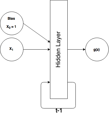
Here, \(t-1\) refers to the previous time step (and e.g. \(t-2\) would refer to 2 time steps ago). Thus, for each time step, we feed the output of the hidden layer from the last time step back into the hidden layer of the current time step. This is how we achieve the memory. It turns out implementing this is actually really simple, and we can do so by re-imagining our network as a feedforward network with some additional input units called contex units. These context units are treated exactly like ordinary input units, with weighted connections to the hidden layer and no activation function. Unlike a normal input unit, however, we aren't supplying the data, the context units simply return the output of \(t-1\)'s hidden layer. In this way, we've just created a feedforward architecture again. Take a look at how the network looks showing all the units:
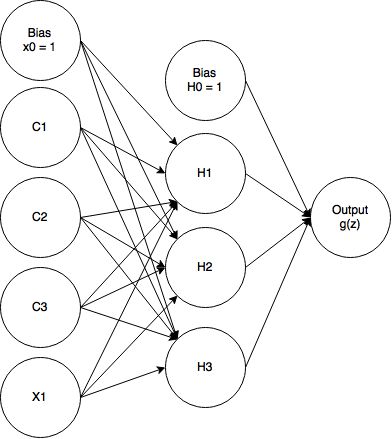
Notice, we only have one real input unit, but we have 3 additional context units (C1 -> C3) that act as inputs and of course we have our bias unit. This type of RNN is called an Elman neural network. There is a similar type of architecture called a Jordan neural network where instead of the context units returning the hidden layer output from \(t-1\), they return the output from the output unit from \(t-1\).
Notice how we have 3 context units and 3 hidden units. That's not a coincidence, an Elman network by definition has the same number of context units as it does hidden units so that each context unit is matched with a corresponding hidden unit. That is, the output from hidden unit 1 (H1) from \(t-1\) is stored and returned by context unit 1 (C1) at the current time step.
Also note that the context units return the hidden output without manipulation. That is, if H1 output 0.843 in the last time step, \(t-1\), then C1 will save that exactly, and use that as its output in the current time step, \(t\). Of course the value 0.843 will be sent over to the hidden layer after it's been weighted.
The reason I chose 3 hidden units is just a matter of training performance. 2 units works too but has a harder time training.
Since we've re-imagined the RNN's recurrent connections as a feedforward network with some additional inputs, we can train it exactly the same way we would any other feedforward NN (FFNNs): backpropagation and gradient descent. The only difference is that training RNNs happens to be much more difficult than FFNNs for reasons I won't detail here. Modern RNN implementations like the Long Short Term Memory (LSTM) networks laregely solve this training problem with additional complexities.
So that's actually all the theory behind our simple RNN. It's really not much more complicated than a feedforward network. Let's get to work..
Let's build it, in Julia, a few lines at a time
X = [0,0,1,1,0,1,0,0,1,1,0,1,0]
Y = [0,0,0,1,1,0,1,0,0,1,1,0,1];
Here I've simply defined our input \(X\) vector and our expected output \(Y\) vector. I arbitrarily chose a sequence of 1s and 0s for the \(X\) vector and then manually computed the LEFTBIT of each consecutive pair of bits and stored those in the \(Y\) vector. Remember that I chose to keep the Y vector the same length as the X vector by adding a 0 in the beginning, but for the purposes of training, we will ignore the first output of the network since it can't compute the LEFTBIT of only one bit.
Note: These are both column vectors. We will not be using the entire \(X\) vector as an input. We will access the each element of the \(X\) vector in order and feed those one by one into our network. We will refer to the corresponding element in our \(Y\) vector to calculate the error of our network.
numIn, numHid, numOut = 1, 3, 1;
Here I define some variables that control how many input units, hidden layer units, and output units our network has. You can change the number of hidden units without having to modify anything else and see how it affects performance. You can't change the number of input or output units without also changing how we structure the input and output data.
theta1 = 2 * randn( numIn + numHid + 1, numHid )
theta2 = 2 * randn( numHid + 1, numOut )
theta1_grad = zeros(numIn + numHid + 1, numHid)
theta2_grad = zeros(numHid + 1, numOut);
First, I'm randomly initializing our weight vectors (I tend to use the terms "weights" and "theta" interchangeably. theta1 and theta2 are the weights for the input-to-hidden layer and hidden-to-output layer, respectively.)
I'm initializing the theta vectors by using the randn() function that returns an array of random values from the normal distribution. I've scaled up these random numbers a bit by multiplying by 2. There is no right way to initialize weights, only wrong ways. People try all sorts of different methods. I've chosen this way because it works relatively well for this particular NN and because it's simple. There are much more complicated ways to initialize weights that may work better. The general wisdom here is to make the weights random and well-distributed but constrained within the limits of what makes sense for the particular neural network (often from trial and error).
The second block is to intitialize our gradient vectors to zero vectors, which will store and accumulate the gradients during backpropagation.
epochs = 60000
alpha = 0.1
epsilon = 0.3;
Some additional parameters for the backpropagation training. Epochs refers to the number of iterations we will train. Yes, 60000 is a big number but RNNs are hard to train. We want to train until the network's error stops decreasing.
alpha is our learning rate (i.e. how big each gradient descent step is). epsilon is our momentum rate. We will be using the momentum method as part of our gradient descent implementation which I will explain in further detail below. Note that I set these constants from trial and error.
hid_last = zeros(numHid, 1)
last_change1 = zeros(numIn + numHid + 1, numHid)
last_change2 = zeros(numHid + 1, numOut)
m = size(X,1) # m = the number of elements in the X vector;
hid_last is a vector that will store the output from the hidden layer units for use in the next time step. We just initialize to zeros at first.
last_change1 and last_change2 are for the momentum learning. In momentum learning, we attempt to prevent gradient descent from getting stuck in local optima by giving the weight updates momentum, e.g. if a weight is rapidly decreasing at one point, we will try to keep it going in that same direction by making the next weight update take into account the previous weight update. These vectors simply store the weight updates from the previous iteration. The simplest implementation of gradient descent-based weight updates uses this equation:
where \(\theta_j\) refers to a particular weight, \(\alpha\) is the learning rate, and \(\frac{\partial C}{\partial \theta_j}\) is the gradient of the cost function \(C\) for that particular weight, \(\theta_j\).
With momentum, the weight update takes this form:
Where all notation remains the same, except that \(\epsilon\) is our momentum rate and \(\Delta_{t-1}\theta_j\) refers to the weight change from the previous iteration. Thus, how much we change the weight this iteration partially depends on how much we changed the weight last iteration. And we can scale this term up or down by changing \(\epsilon\)
function sigmoid(z)
    return 1.0 ./ (1.0 + exp(-z))
end;
This will define the sigmoid activation function we will use for our neurons. Should be fairly self-explanatory.
Now let's get to the meat of our training code:
for i = 1:epochs
    #forward propagation
    s = rand(1:(m-1)) #random number between 1 and number of elements minus 1
    for j = s:m #for every training element
        y = Y[j,:] #set our expect output, y, to be the corresponding element in Y vector
        context = hid_last #update our context units to hold t-1's hidden layer output
        x1 = X[j,:] #our single input value, from the X vector
        a1 = [x1, context, 1] #add context units and bias unit to input layer; 5x1 vector
        z2 = theta1' * a1 #theta1 = 5x3, a1 5x1. So theta1' * a1 = 3x5 * 5x1 = 3x1 vector
        a2 = [sigmoid(z2), 1] #calculate output, add bias to hidden layer;
        hid_last = a2[1:end-1,1] #store the output values for next time step, but ignore bias
        z3 = theta2' * a2 #theta2 = 4x1, a2 = 4x1. So theta2' * a2 = 1x4 * 4x1 = 1x1 vector
        a3 = sigmoid(z3) #compute final output
        #Ignore first output in training
        if j != s
            #calculate delta errors
            d3 = (a3 - y);
            d2 = (theta2 * d3) .* (a2 .* (1 - a2))
            #accumulate gradients
            theta1_grad = theta1_grad + (d2[1:numHid, :] * a1')';
            theta2_grad = theta2_grad + (d3 * a2')'
        end
    end
    #calculate our weight updates
    theta1_change = alpha * (1/m)*theta1_grad + epsilon * last_change1;
    theta2_change = alpha * (1/m)*theta2_grad + epsilon * last_change2;
    #update the weights
    theta1 = theta1 - theta1_change;
    theta2 = theta2 - theta2_change;
    #store the weight updates for next time (momentum method)
    last_change1 = theta1_change;
    last_change2 = theta2_change;
    #reset gradients
    theta1_grad = zeros(numIn + numHid + 1, numHid);
    theta2_grad = zeros(numHid + 1, numOut);
end
If you've gone through my tutorial on backpropagation and gradient descent, most of this code will look very familiar so I'm not going to explain every single line. I've also commented it well. But let's go over the important/new parts of the code.
s = rand(1:(m-1))
For every training iteration, we initialize s to be a random number between 1 and (m - 1) where m is the number of elements in \(X\). This is sort of a mini-batch, stochastic gradient descent implementation because we're training on a random subset of our input sequence each training iteration. This will hopefully ensure our network learns how to actually compute LEFTBIT and not just memorize the original sequence we gave it to train on (which would be overfitting).
context = hid_last
x1 = X[j,:]
a1 = [x1, context, 1]
This is where we build up our input layer. First we get the element from the input \(X\) vector that we're currently training on and add it to our input layer \(a1\), then we add in our context units, and finally add in the bias value of 1. The rest is ordinary feedforward logic.
hid_last = a2[1:end-1,1]
We save the current hidden layer output in the hid_last vector that we defined and initialized outside of the training loop.
if j != s
this block calculates the network deltas and gradients (backpropagation) but not if this is the first element in the sequence because the network can't compute LEFTBIT on only 1 input bit. Thus is wouldn't make sense to calculate an error for the first bit when it's impossible for the RNN to get it correct.
theta1_change = alpha * (1/m)*theta1_grad + epsilon * last_change1;
theta2_change = alpha * (1/m)*theta2_grad + epsilon * last_change2;
theta1 = theta1 - theta1_change;
theta2 = theta2 - theta2_change;
This is where we calculate the weight updates based on the learning rate alpha, the gradients, and the previous weight update (momentum method).
To continue with the momentum method in the next iteration, we save how much we updated the weights in this iteration in our last_change vectors:
last_change1 = theta1_change
last_change2 = theta2_change
theta1_grad = zeros(numIn + numHid + 1, numHid);
theta2_grad = zeros(numHid + 1, numOut);
Here we reset the gradients for the next epoch (and thus training 'mini-batch'). We don't want to keep accumulating gradients forever. We reset them after accumulating gradients for each training sequence.
Okay, so that is how we implement and train our simple RNN to compute LEFTBIT on an arbitrary binary sequence.
After training it, let's run the network forward over a new binary sequence to see if it learned.
results = Float64[] #vector to store the output values of the network
Xt = [1,0,0,1,1,0,1] #Arbitrary new input data to test our network
for j = 1:size(Xt,1) #for every training element
    context = hid_last
    x1 = Xt[j,:]
    a1 = [x1, context, 1] #add bias, context units to input layer
    z2 = theta1' * a1
    a2 = [sigmoid(z2); 1] #output hidden layer
    hid_last = a2[1:end-1,1]
    z3 = theta2' * a2
    a3 = sigmoid(z3)
    push!(results, a3[1]) #add current output to results vector
end
println("Results:  "  * string(int(round(results))))
println("Expected: " * string([0,1,0,0,1,1,0]))
Results:  [0,1,0,0,1,1,0]
Expected: [0,1,0,0,1,1,0]
It worked! As you can see our neural network output exactly what we expected. Keep in mind we ignore the first bit in the output vector. Although in this case the network happened to output 0 as the first bit like we defined in our \(Y\) vector, it could have also output 1 and it would still be correct since the rest of the output sequence is indeed the computed LEFTBIT of each sequential pair of bits in our input vector.
I literally copy and pasted the code from above in our training code to just run the network forward but added a results vector to store the sequence of output results.
Closing Words...
Hopefully this was easy to follow. This was really a bare-bones implementation of a simple recurrent neural network (other than the fact we added in the momentum method to help it learn better). To take this further, I suggest you try defining a cost function (e.g. the cross-entropy cost function) and graph the cost versus the epochs. Then you can vary the hyperparameters of the network (e.g. $\alpha, \epsilon, $ the number of hidden units, etc) and see how it effects the gradient descent.
I also really hope you can appreciate the beauty and value of Julia as a language for modern scientific computing. I will continue to write articles using Python but will likely increasingly use Julia.
As always, please email me (outlacedev@gmail.com) to let me know about errors or if you have other comments or questions.
References:
- https://www.youtube.com/watch?v=e2sGq_vI41s
- http://iamtrask.github.io/2015/07/12/basic-python-network/