Δ ℚuantitative √ourney

Persistent Homology (Part 3)

Topological Data Analysis - Part 3 - Persistent Homology

This is Part 3 in a series on topological data analysis. See Part 1 | Part 2 | Part 4 | Part 5

In this part we begin to apply our the math we learned from Parts 1-2 to actually calculating the interesting topological features of a simplicial complex.

Back to simplicial homology

We've finally covered enough group theory to be able to finish our calculations of homology groups on simplicial complexes. As you should recall, we had given definitions for the n-th homology group and the n-th Betti numbers.

Betti number's are what we ultimately want. They nicely summarize the topological properties of a simplicial complex. If we have a simplicial complex that forms a single circular object, then \(b_0\) (the 0th Betti Number) represents the number of connected components which is 1, \(b_1\) is the number of 1-dimensional holes (i.e. cycles) which is 1, and \(b_n, n \gt 1\) are the higher-dimensional holes of which there are zero.

Let's see if we can calculate the Betti Numbers of a simple triangle simplicial complex.

Recall that \(\mathcal T = \text{ {{a}, {b}, {c}, [a, b], [b, c], [c, a]} }\). (Depicted below).

Since we know, by visual inspection, that \(T\) should have Betti numbers \(b_0 = 1\) (1 connected component), \(b_1 = 1\) (1 one-dimensional hole), we will only compute those Betti numbers.

Let's walk through the whole sequence of steps slowly. First we'll note the n-chains.

The 0-chain is the set of 0-simplices: \(\text{ {{a}, {b}, {c} } }\) The 1-chain is the set of 1-simplices: \(\text{ [a, b], [b, c], [c, a] }\) There are no higher-dimensional n-chains.

Now we can use the n-chains to define our chain groups. We're going to be using coefficients from \(\mathbb Z_2\), which is a field, and remember there are only 2 elements \(\{0,1\}\) where \(1+1=0\).

The 0-chain group is defined as:

Remember a group only has an addition operation defined but we're building the group by using a multiplication operation from the field \(\mathbb Z_2\). So this group is actually isomorphic to \(\mathbb Z_{2}^{3} = Z_{2} \oplus Z_{2} \oplus Z_{2}\).

But we also want to represent our chain groups as a vector space. This means it becomes a structure where elements can be scaled up or down (i.e. multiplication operation) by elements of a field (in our case \(\mathbb Z_2\)) and added together, with all results still contained in the structure. If we only pay attention to the addition operation then we're basically looking at its group structure, whereas if we pay attention to both the multiplcation and addition operations then we are considering it as a vector space.

0-chain vector space is generated by:

(Yes it's the same set that forms the group from above).

The vector space is the set of elements we can multiply by 0 or 1, and add them together. For example, we can do: \(1*(a,0,0) + 1*(0,0,c) = (a,0,c)\). This vector space is so small \((2^3=8\ \text{elements})\) we can actually list out all the elements. Here they are:

You can see that we can add any two elements in this vector space and the result will be another element in the vector space. A random example: \((a,0,c) + (a,b,c) = (a+a,0+b,c+c) = (0,b,0)\). Recall addition is component-wise. We can also multiply vectors by an element in our field \(\mathbb Z_2\) but since our field is finite with only 2 elements, it's not very interesting, e.g. \(1*(a,b,0) = (a,b,0)\) and \(0*(a,b,0) = (0,0,0)\), but none the less, the multiplication operation still results in an element within our vector space.

We can represent this vector space as a polynomial, so our 0-chain vector space can be defined equivalently as:

We can easily translate a polynomial like \(a+b+c\) to its ordered-set notation \((a,b,c)\). Or \(a+b\) is \((a,b,0)\). The vector space seen as a set of polynomials looks like this:

It's more convenient to work with the polynomial form, in general, because we can make familiar algebraic equations like

(Recall that the inverse of an element in \(\mathbb Z_2\) is just itself, hence \(-b = b\) where "\(-\)" denotes inverse).

NOTE: It is very important to keep track of whether we're talking about groups or vector spaces. I will use a normal letter \(C\) to denote the chain group and the fancy script \(\mathscr{C}\) to denote the chain (vector) space. They have the same underlying set, only different operations defined. If we talk about the group form we can only reference its addition operation, whereas if we talk about its vector space form we can talk about its multiplication and addition operation.

Let's do the same for the 1-chains: \(\text{ [a, b], [b, c], [c, a] }\). We can use the 1-chain set to define another chain group, \(C_1\). It will be isomorphic to \(C_0\) and hence \(\mathbb Z_{2}^{3}\).

We can define a vector space, \(\mathscr C_1\), using this chain group in the same way we did for \(C_0\). I will use the polynomial form henceforth. Remember, the chain group and vector space have the same set, its just that the vector space has two binary operations instead of one.

This is the full list of elements in the vector space:

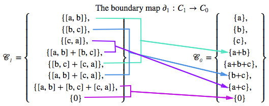
Just for clarification about the boundary map, here is a diagram of it. This shows how the boundary operator maps each element in \(C_1\) to an element in \(C_0\).

Now we can start computing the first Betti number, \(b_0\).

Recall the definition of a Betti number is:

The n-th Betti number, \(b_n = dim(H_n)\), where \(H_n\) is the n-th homology group.

And recall the definition of a homology group

The \(n^{th}\) Homology Group \(H_n\) is defined as \(H_n\) = Ker \(\partial_n \ / \ \text{Im } \partial_{n+1}\).

Lastly, recall the definition of a kernel:

The kernel of \(\partial(C_n)\), denoted \(\text{Ker}(\partial(C_n))\) is the group of \(n\)-chains \(Z_n \subseteq C_n\) such that \(\partial(Z_n) = 0\)

So first we need the kernel of the boundary of \(C_0\), Ker \(\partial(C_0)\). Remember the boundary map \(\partial\) gives us a map from \(C_n \rightarrow C_{n-1}\).

In all cases, the boundary of a 0-chain is \(0\), thus the Ker \(\partial(C_0)\) is the whole 0-chain.

This forms another group we will denote \(Z_0\) (or \(Z_n\) generally), the group of 0-cycles, which in general is a subgroup of \(C_0\), i.e. \(Z_n \leq C_n\). With addition defined over \(\mathbb Z_2\) then \(Z_0\) is also ismorphic to \(\mathbb Z_2\) and hence is the same as \(C_0\).

The other thing we need to find the homology group \(H_0\) is \(\text{Im } \partial_{1}\). This forms a subgroup of \(Z_0\) that we denote \(B_0\) (or more generally \(B_n\)) which is the group of boundaries of the (n+1)-chain. Hence, \(B_n \leq Z_n \leq C_n\).

So \(\text{Im } \partial_{1} = {0}\)

Thus we compute the quotient group \(H_0 = Z_0\ /\ B_0\), which in this case is:

so we take the left cosets of \(\{0\}\) for the two elements in \(Z_0\) to get the quotient group, which gives us:

So in general, if \(B_n = \{0\}\) then \(Z_n\ /\ B_n = Z_n\). Hence \(H_0 = Z_0\).

The Betti number \(b_0\) is the dimension of \(H_0 = Z_0\). What is the dimension of \(H_0\)? Well, it has two elements, but the dimension is defined as the smallest set of generators for a group, and since this group is isomorphic to \(\mathbb Z_2\), it only has 1 generator. For \(\mathbb Z_2\) the generator is \(1\), since the whole group can be formed by repeatedly applying the addition operation on \(1\), i.e. \(1+1=0, 1+1+1 = 1\) and now we have the full \(\mathbb Z_2\).

So \(b_0 = dim(H_0) = 1\), which is what we expected, this simplicial complex has 1 connected component.

Now let's start calculating Betti \(b_1\) for the 1-dimension. This time it will be a bit different because figuring out \(\text{Ker}\partial(C_1)\) is going to be more involved. We're going to need to do some algebra.

So, we first want \(Z_1\), the group of 1-cycles. This is the set of 1-simplices whose boundary is 0. Remember the 1-chain is \(\{ [a,b], [b,c], [c,a]\}\) and forms the 1-chain group \(C_1\) when applied over \(\mathbb Z_2\). We will setup an equation like this:

For this equation to be satisfied, then all the coefficients \(\lambda_n\) for each term need to sum to 0 to make \(a,b,c\) go to \(0\). That is, if the whole equation goes to \(0\), then each term like \(a(\lambda_0 + \lambda_2) = 0\), hence $(\lambda_0 + \lambda_2) = 0, $. So now we basically have a system of linear equations:

Now, let's go back to the general expression for the 1-chain vector space \(\mathscr C_1 = \lambda_0([a,b]) + \lambda_1([b,c]) + \lambda_2([c,a])\). When we take the boundary of that and set it to 0, we get \(\lambda_0 = \lambda_1 = \lambda_2\), and I proposed we just replace those with one symbol, \(\phi\).

Hence, the cycle group:

So the cycle group only contains two elements and is hence isomorphic to \(\mathbb Z_2\).

NOTE: I will introduce new notation. If two mathematical structures (e.g. groups) \(G_1, G_2\) are isomorphic, we denote it as \(G_1 \cong G_2\)

If \(\phi = 0\), then we get \(\phi([a,b] + [b,c] + [c,a]) = 0([a,b] + [b,c] + [c,a]) = 0 \\\) , whereas if \(\phi = 1\), then \(\phi([a,b] + [b,c] + [c,a]) = 1([a,b] + [b,c] + [c,a]) = [a,b] + [b,c] + [c,a] \\\) So the full group is:

The boundary group \(B_1 = Im\partial(C_2)\) but since \(C_2\) is an empty set, \(B_1 = \{0\}\).

So once again we can compute the homology group:

And Betti \(b_1 = dim(H_1) = 1\) since we only have one generator in the group \(H_1\).

So that's it for that very simple simplicial complex. We'll move on to a bigger complex. This time I won't be as verbose and will use a lot of the simplifying notation and conventions that I've already defined or described.

Let's do the same but with a slightly more complicated simplicial complex that we've seen before:

(Depicted below).

Notice we now have a 2-simplex [a, b, c], depicted as the filled in triangle.

This time we will use the full integer field \(\mathbb Z\) for our coefficients, thus the resulting vector spaces will be infinite instead of finite spaces that we could list out. Since we're using \(\mathbb Z\), we must define what it means to be a "negative" simplex, e.g. what does \(-[c,a]\) mean? Well we discussed this previously. Basically we define two ways a simplex can be oriented and opposite orientation to the original definition will be assigned the "negative" value of a simplex.

So \([a,c] = -[c,a]\). But what about \([a,b,c]\)? There are more than two ways to permute a 3 element list, but there only two orientations.
If you look at the oriented simplex from before: There are only two ways you can "go around" the loop. Either clockwise or counterclockwise.
\([a,b,c]\) is clockwise (and we'll call it positive).
\([c,a,b]\) is also clockwise (so \([c,a,b] = [a,b,c]\))
\([a,c,b]\) is a counterclockwise, as well as \([b,c,a]\), so \([a,b,c] = [c,a,b] = -[a,c,b] = -[b,c,a]\).

Let's start by listing our chain groups.

Recall the angle brackets mean span, i.e. the set of all linear combinations of the elements between the angle brackets. This is obviously much more succinct than how we we're building the groups in our last example. And note how each group is isomorphic to the vector space \(\mathbb Z^n\) where \(n\) is the number of simplices in the n-chain.

We can thus describe our chain complex as:

We know, since we can easily visualize the simplicial complex, that it has one connected component and one 1-cycle (one 1-dimensional hole). Hence, Betti \(b_0 = 1, b_1 = 1\). But we need to calculate that for ourselves.

Let's start from the higher-dimensional chain group, the 2-chain group.

Remember, \(Z_n = \text{Ker}\partial(C_n)\) the group of n-cycles, which is a subgroup of \(C_n\). And \(B_n = \text{Im}\partial(C_{n+1})\) is the group of n-boundaries, which is a subgroup of the n-cycles. Hence \(B_n \leq Z_n \leq C_n\). Also recall, the homology group \(H_n = Z_n\ /\ B_n\) and the n-th Betti number is the dimension of the n-th homology group.

To find \(Z_n\), we have to setup our expression for a general element in \(C_n\).

Since there are no 3-simplices or higher, \(B_2 = {0}\). Thus Betti \(b_2 = dim(\{0\} / \{0\}) = 0\). This is what we expect, there are no 2-dimensional holes in the simplicial complex.

Let's do the same for \(C_1\).

Now to get the boundaries \(B_1 = Im\partial(C_2)\).

Another way to more easily take the quotient group \(H_1 = Z_1\ /\ B_1\) is to just pay attention to what \(Z_n, B_n\) are isomorphic to in terms of \(\mathbb Z^n\). In this case:

So since \(H_1 \cong \mathbb Z\), the Betti number for \(H_1\) is 1 because the dimension of \(\mathbb Z\) is 1 (it only has one generator or basis).

So I think you get the point by now, I'm not going to go through all the details of calculating Betti \(b_0\), it should be 1 since there is only one connected component.

Next time...

We've learned how to calculate homology groups and Betti numbers of simple simplicial complexes by hand. But we're going to need to develop some new tools so that we can let computer algorithms handle these calculations for the real, and generally much larger, simplicial complexes. Next time we'll see how linear algebra gives us an efficient means of doing this.

References (Websites):

1. http://dyinglovegrape.com/math/topology_data_1.php
2. http://www.math.uiuc.edu/~r-ash/Algebra/Chapter4.pdf
3. https://en.wikipedia.org/wiki/Group_(mathematics)
4. https://jeremykun.com/2013/04/03/homology-theory-a-primer/
5. http://suess.sdf-eu.org/website/lang/de/algtop/notes4.pdf
6. http://www.mit.edu/~evanchen/napkin.html

References (Academic Publications):

1. Basher, M. (2012). On the Folding of Finite Topological Space. International Mathematical Forum, 7(15), 745–752. Retrieved from http://www.m-hikari.com/imf/imf-2012/13-16-2012/basherIMF13-16-2012.pdf

2. Day, M. (2012). Notes on Cayley Graphs for Math 5123 Cayley graphs, 1–6.

3. Doktorova, M. (2012). CONSTRUCTING SIMPLICIAL COMPLEXES OVER by, (June).

4. Edelsbrunner, H. (2006). IV.1 Homology. Computational Topology, 81–87. Retrieved from http://www.cs.duke.edu/courses/fall06/cps296.1/

5. Erickson, J. (1908). Homology. Computational Topology, 1–11.

6. Evan Chen. (2016). An Infinitely Large Napkin.

7. Grigor’yan, A., Muranov, Y. V., & Yau, S. T. (2014). Graphs associated with simplicial complexes. Homology, Homotopy and Applications, 16(1), 295–311. http://doi.org/10.4310/HHA.2014.v16.n1.a16

8. Kaczynski, T., Mischaikow, K., & Mrozek, M. (2003). Computing homology. Homology, Homotopy and Applications, 5(2), 233–256. http://doi.org/10.4310/HHA.2003.v5.n2.a8

9. Kerber, M. (2016). Persistent Homology – State of the art and challenges 1 Motivation for multi-scale topology. Internat. Math. Nachrichten Nr, 231(231), 15–33.

10. Khoury, M. (n.d.). Lecture 6 : Introduction to Simplicial Homology Topics in Computational Topology : An Algorithmic View, 1–6.

11. Kraft, R. (2016). Illustrations of Data Analysis Using the Mapper Algorithm and Persistent Homology.

12. Lakshmivarahan, S., & Sivakumar, L. (2016). Cayley Graphs, (1), 1–9.

13. Liu, X., Xie, Z., & Yi, D. (2012). A fast algorithm for constructing topological structure in large data. Homology, Homotopy and Applications, 14(1), 221–238. http://doi.org/10.4310/HHA.2012.v14.n1.a11

14. Naik, V. (2006). Group theory : a first journey, 1–21.

15. Otter, N., Porter, M. A., Tillmann, U., Grindrod, P., & Harrington, H. A. (2015). A roadmap for the computation of persistent homology. Preprint ArXiv, (June), 17. Retrieved from http://arxiv.org/abs/1506.08903

16. Semester, A. (2017). § 4 . Simplicial Complexes and Simplicial Homology, 1–13.

17. Singh, G. (2007). Algorithms for Topological Analysis of Data, (November).

18. Zomorodian, A. (2009). Computational Topology Notes. Advances in Discrete and Computational Geometry, 2, 109–143. Retrieved from http://citeseerx.ist.psu.edu/viewdoc/summary?doi=10.1.1.50.7483

19. Zomorodian, A. (2010). Fast construction of the Vietoris-Rips complex. Computers and Graphics (Pergamon), 34(3), 263–271. http://doi.org/10.1016/j.cag.2010.03.007

20. Symmetry and Group Theory 1. (2016), 1–18. http://doi.org/10.1016/B978-0-444-53786-7.00026-5