Δ ℚuantitative √ourney

Persistent Homology (Part 4)

Topological Data Analysis - Part 4 - Persistent Homology

This is Part 4 in a series on topological data analysis. See Part 1 | Part 2 | Part 3 | Part 5

In this part we learn more about how linear algebra can help us calculate topological features in a computationally efficient manner.

Linear algebra saves the day

You might have noticed that calculating the homology groups and Betti numbers by hand can be very tedious and impractical for anything larger than the simple examples we've considered thus far. Fortunately, there are better ways. In particularly, we can represent most of the computation of homology groups in terms of vectors and matrices and computers are very efficient when working with vectors and matrices.

Now, we already went over what a vector is (an element in a vector space) but what is a matrix? You probably think of a matrix has a kind of 2-dimensional grid of numbers, and you know you can multiply matrices by other matrices and vectors and what not. Well a grid of numbers is certainly a convenient notation for matrices, but that's not what they are.

What's a matrix?

By this point, you should be comfortable with the idea of a function or map. These are both ways of translating one type of mathematical structure into another (or at least mapping one element in a structure to a different element in the same structure). In particular, we've spent a good amount of time working with boundary maps that mapped a higher-dimensional chain group to a lower dimensional chain group that preserved the structure of the original group in some way (it is a homomorphism).

So just like we can have a map between two groups, we can have a map between two vector spaces. And we call (linear) maps between vector spaces, matrices. A matrix basically applies a linear transformation on a vector space (or individual vector element) producing new vector space. A linear transformation just implies that we can only transform the vector space via the normal vector operations of scaling by a constant and addition of a constant vector.

Definition (Linear Tansformation)
More precisely, a linear transformation \(M\ :\ V_1 \rightarrow V_2\) is a map \(M\) from the vector spaces \(V_1\) to \(V_2\) such that \(M(V_1 + V_2) = M(V_1) + M(V_2)\) and \(M(aV_1) = aM(V_1)\) where \(a\) is a scalar.

Let's say we want to map the real-valued volume \(\mathbb R^3\) to the plane \(\mathbb R^2\).

Now, what if I want to map \(V_1\) to \(V_2\), that is, I want to send every point in \(V_1\) to a point in \(V_2\). There are many reasons why I might want to do something like this. If I'm making a graphics application, for example, I want to offer an option to rotate images drawn, and this is simply a matter of applying a linear transformation on the pixels.

So we want a map \(M : V_1 \rightarrow V_2\), and we'll call this map a matrix. Notice that \(V_1\) has a basis with 3 elements, and \(V_2\) has a basis with 2 elements. In order to map from one space to the other, we just need to map one basis set to another basis set. And remember, since this is a linear map, all we are allowed to do to a basis is multiply it by a scalar or add another vector to it; we can't do exotic things like square it or take the logarithm.

Let's call the 3 basis elements of \(V_1: B_1, B_2, B_3\). Hence, \(V_1 = \langle{B_1, B_2, B_3}\rangle\). Similarly, we'll call the 2 basis elements of \(V_2: \beta_1, \beta_2\). Hence, \(V_2 = \langle{\beta_1, \beta_2}\rangle\). (Remember the angle brackets \(\langle\rangle\) mean span, i.e. the set of all linear combinations of those elements). We can setup equations such that any vector in \(V_1\) can be mapped to a vector in \(V_2\) by using the fact that each vector space can be defined by their bases.

New Notation (Vector)
To prevent confusion between symbols that refer to scalars and symbols that refer vectors, I will henceforth add a little arrow over every vector \(\vec{v}\) to denote it is a vector, not a scalar. Remember, the scalar is just a single element from the underlying field \(F\) over which the vector space is defined.

We can define our map \(M(V_1) = V_2\) in this way:

That is, the map from each basis in \(V_1\) is setup as a linear combination of the basis elements in \(V_2\). This requires us to define a total of 6 new pieces of data: \(a,b,c,d,e,f \in \mathbb R\) required for our mapping. We just have to keep track of the fact that \(a,b\) are for mapping to \(\beta_1\) and \(d,e,f\) are for mapping to \(\beta_2\). What's a convenient way to keep track of all of that? Oh I know, a matrix!

That is a very convenient way to represent our map \(M\ :\ V_1 \rightarrow V_2\) indeed. Notice that each column of this matrix corresponds to the "mapping equation" coefficients for each M(B_n). Also notice that the dimensions of this matrix, \(2\times3\), corresponds to the dimensions of the two vector spaces we're mapping to and from. That is, any map \(\mathbb R^n \rightarrow \mathbb R^m\) will be represented as an \(m\times n\) matrix. It is important to keep in mind that since the linear map (and hence the matrix) depend on coefficients applied to a basis, then the matrix elements will change if one uses a different basis.

Knowing this we can easily see how vector-matrix multiplication should work and why the dimensions of a matrix and vector have to correspond. Namely, a \(n \times m\) vector/matrix multiplied by a \(j \times k\) vector/matrix must produce a \(n \times k\) vector/matrix, and for it to work at all, \(m = j\).

This is how we can multiply our matrix map \(M\) by any vector in \(V_1\) to produce the mapped-to vector in \(V_2\):

Ok now we know a matrix is a linear map between two vector spaces. But what happens if you multiply two matrices together? Well that is just a composition of maps. For example, we have three vector spaces \(T, U, V\) and two linear maps \(m_1, m_2\):

To get from \(T\) to \(V\), we need to apply both maps: \(m_2(m_1(T)) = V\). Hence, multiplying two matrices together gives us a composition of maps \(m_2 \circ m_1\). The identity matrix is an identity map (i.e. it doesn't change the input) that takes the form where 1s are along the diagonal and 0s everywhere else, e.g.:

Back to simplicial homology (again)

We learned all of that so we can represent the boundary map \(\partial(C_n)\) as a matrix so we can apply the tools of linear algebra. This makes sense since we already know that the chain groups \(C_n\) can be viewed as vector spaces when we allow scalar multiplication, so then a linear map between the chain vector spaces is the boundary map, that we can represent as a matrix.

We represent an \(n\)-boundary map, i.e. \(\partial(C_n)\), where \(n\) is the dimension of the chain group, \(k\) is the number of simplices in \(C_n\) and \(l\) is the number of simplices in \(C_{n-1}\), as a matrix with \(k\) columns and \(l\) rows. Thus each column represents a simplex in \(C_n\) and each row represents a simplex in \(C_{n-1}\). We put a \(1\) in a cell of the matrix if the simplex in that column maps to the simplex in that row. For example, \(\partial([a,b]) = a - b\) if the field is \(\mathbb Z\), so we will put a \(1\) in the row for \(a\) and \(b\) since the 1-simplex \([a,b]\) maps to those two 0-simplices.

Let's try calculating the homology groups of the previous simplicial complex (depicted below again) using matrices and vectors. We're going to go back to using \(\mathbb Z_2\) as our field (so simplex orientation can be ignored) because it is computationally more efficient to do so.

Since we're using the (very small) finite field \(\mathbb Z_2\) then we can actually list out all the vectors in our chain (group) vector space. We have 3 chain groups, namely the group of 0-simplices (vertices), 1-simplices (edges), and 2-simplices (triangle).

In our example, we only have a single 2-simplex: [a,b,c], thus the group it generates over the field \(\mathbb Z_2\) is only \(\{0, [a,b,c]\}\) which is isomorphic to \(\mathbb Z_2\). Recall, in general, the group generated by the number \(n\) of \(p\)-simplices in a simplicial complex is isomorphic to \(\mathbb Z^n_2\). For a computer to understand, we can encode the group elements just using their coefficients 1 or 1. So, for example, the group generated by \([a,b,c]\) can just be represented as \(\{0,1\}\). Or the group generated by the 0-simplices \(\{a, b, c, d\}\) can be represented by 4-dimensional vectors, for example, if a group element is \(a+b+c\) then we encode this as \((1, 1, 1, 0)\) where each position represents the presence or abscence of \((a, b, c, d)\), respectively.

Here are all the chain groups represented as vectors with just coefficients (I didn't list all elements for \(C_1\) since there are so many [32]):

To represent the boundary map (which is a linear map) of the group of \(p\)-simplices as a matrix, we set the columns to represent each \(p\)-simplex in the group, and the rows represent each \((p-1)\)-simplex. We put a \(1\) in each position of the matrix if the \((p-1)\)-simplex row is a face of the \(p\)-simplex column.

We index rows and columns as an ordered pair \((i, j)\) respectively. Thus the element \(a_{2,3}\) is the element in the 2nd row (from the top) and the 3rd column (from the left).

The generic boundary matrix is thus (each column is a \(p\)-simplex, each row is a \((p-1)\)-simplex):

We'll start by representing the boundary map \(\partial(C_2)\) as a matrix. There's only one 2-simplex in \(C_2\) so there is only one column, but there are five 1-simplices in \(C_1\) so there are 5 rows.

We put a \(1\) if each row-element was a face of the simplex \([a,b,c]\). This matrix makes sense as a linear map because if we multiply it by a vector element in \(C_2\) (there's only 1, besides the 0 element) we get what we expect:

Okay, let's move on to building the boundary matrix \(\partial(C_1)\):

Does this make sense? Let's check with some python/numpy. Let's take an arbitrary element from the group of 1-chains, namely: \([a,b]+[c,a]+[c,d]\) which we've encoded as \((1,0,1,1,0)\) and apply the boundary matrix and see what we get.

import numpy as np
b1 = np.matrix([[1,0,1,0,0],[1,1,0,0,1],[0,1,1,1,0],[0,0,0,1,1]]) #boundary matrix C_1
el = np.matrix([1,0,1,1,0]) #random element from C_1
np.fmod(b1 * el.T, 2) # we want integers modulo 2

matrix([[0],
        [1],
        [0],
        [1]])

\(\require{cancel}\)

Recall that \((0,1,0,1)\) translates to \(b+d\). By hand we can calculate the boundary and compare:

It works!

Lastly, we need the boundary matrix for \(C_0\) which is trivial since the boundary of \(0\)-simplices always maps to \(0\), so

Okay, now we have our three boundary matrices, how do we calculate the Betti numbers? Well recall that sequence of subgroups of a chain group: $ B_n \leq Z_n \leq C_n $ which are the group of boundaries, group of cycles, and chain group, respectively.

Also recall that Betti \(b_n = dim(Z_n\ /\ B_n)\). But that's when things were represented as just sets with group structure, now everything is represented as vectors and matrices, so instead we define the Betti number \(b_n = rank(Z_n)\ -\ rank(B_n)\). What does rank mean? Rank and dimension are related but not the same. If we think of the columns of a matrix as a set basis vectors: \(\beta_1, \beta_2, \dots \beta_k\) then the dimension of the span of those column vectors \(\langle \beta_1, \beta_2, \dots \beta_k \rangle\) is the rank of the matrix. It turns out that you can also use the rows and it will have the same result. Importantly, however, dimension is defined on the smallest set of basis elements, i.e. the basis elements that are linearly independent.

The boundary matrix \(\partial_n\) contains the information for the chain group and cycles subgroup, and the \(B_{n-1}\) boundary subgroup, all the information we need to calculate the Betti number. Unfortunately, in general, our naïve approach of building the boundary matrix is not in a form where the group and subgroup information is readily accessible. We need to modify the boundary matrix, without disturbing the mapping information it contains, into a new form called Smith normal form. Basically, the smith normal form of a matrix will have \(1\)s along the diagonal starting from the top left of the matrix and \(0\)s everywhere else.

For example,

Notice the \(1\)s along the diagonal do not necessarily need to extend all the way down to the bottom right. And here's the information available once it's in Smith normal form (the red diagonal box indicates the \(1\)s): (Source: "COMPUTATIONAL TOPOLOGY" by Edelsbrunner and Harer, pg. 104)

So how do we get a matrix into Smith normal form? We do so by playing a game involving manipulating the matrix according to some rules. Here are the two allowed operations on the matrix: 1. You can swap any two columns or any two rows in the matrix. 2. You can add a column to another column, or a row to another row.

Now you just need to apply these operations until you get the matrix in Smith normal form. I should point out that this process is alot easier when we use the field \(\mathbb Z_2\). Let's try it out on the boundary matrix for \(C_1\).

We already have 1s across the diagonal, but we have a lot of 1s not along the diagonal.
Steps: Add column 3 to 5, then add column 4 to 5, then add column 5 to 1, then swap columns 1 and 5:

Steps: Add column 1 to 3, add column 2 to 3, swap columns 3 and 4, add row 1 to 2, add row 4 to 2, add row 3 to 2, add row 4 to 3, swap rows 3 and 2, swap rows 4 and 3. Stop.

Once we have the matrix in Smith normal form, we don't do any more operations. We could of course continue adding rows and columns together until we get a matrix of only 0s, but that wouldn't be very helpful! I sort of randomly added rows/columns to get it into the Smith normal form, but there really is an algorithm that can do it relatively efficiently.

Rather than walk through the detailed implementation of the Smith normal form algorithm, I will merely use an existing algorithm:

def reduce_matrix(matrix):
    #Returns [reduced_matrix, rank, nullity]
    if np.size(matrix)==0:
        return [matrix,0,0]
    m=matrix.shape[0]
    n=matrix.shape[1]

    def _reduce(x):
        #We recurse through the diagonal entries.
        #We move a 1 to the diagonal entry, then
        #knock out any other 1s in the same  col/row.
        #The rank is the number of nonzero pivots,
        #so when we run out of nonzero diagonal entries, we will
        #know the rank.
        nonzero=False
        #Searching for a nonzero entry then moving it to the diagonal.
        for i in range(x,m):
            for j in range(x,n):
                if matrix[i,j]==1:
                    matrix[[x,i],:]=matrix[[i,x],:]
                    matrix[:,[x,j]]=matrix[:,[j,x]]
                    nonzero=True
                    break
            if nonzero:
                break
        #Knocking out other nonzero entries.
        if nonzero:
            for i in range(x+1,m):
                if matrix[i,x]==1:
                    matrix[i,:] = np.logical_xor(matrix[x,:], matrix[i,:])
            for i in range(x+1,n):
                if matrix[x,i]==1:
                    matrix[:,i] = np.logical_xor(matrix[:,x], matrix[:,i])
            #Proceeding to next diagonal entry.
            return _reduce(x+1)
        else:
            #Run out of nonzero entries so done.
            return x
    rank=_reduce(0)
    return [matrix, rank, n-rank]

# Source: < https://triangleinequality.wordpress.com/2014/01/23/computing-homology/ >

reduce_matrix(b1)
#Returns the matrix in Smith normal form as well as rank(B_n-1) and rank(Z_n)

[matrix([[1, 0, 0, 0, 0],
         [0, 1, 0, 0, 0],
         [0, 0, 1, 0, 0],
         [0, 0, 0, 0, 0]]), 3, 2]

As you can see we got the same result by hand, but surely the algorithm was more efficient.

Since each boundary map gives us \(Z_n\) (cycles) and \(B_{n-1}\) (boundary for (n-1)-chain group) we need both \(\partial_n\) and \(\partial_{n+1}\) in order to calculate the Betti number for chain group \(n\). Remember, we now calculate Betti numbers as
Betti \(b_n = rank(Z_n) - rank(B_n)\)

Let's start calculating those Betti numbers.

#Initialize boundary matrices
boundaryMap0 = np.matrix([[0,0,0,0]])
boundaryMap1 = np.matrix([[1,0,1,0,0],[1,1,0,0,1],[0,1,1,1,0],[0,0,0,1,1]])
boundaryMap2 = np.matrix([[1,1,1,0,0]])

#Smith normal forms of the boundary matrices
smithBM0 = reduce_matrix(boundaryMap0)
smithBM1 = reduce_matrix(boundaryMap1)
smithBM2 = reduce_matrix(boundaryMap2)

#Calculate Betti numbers
betti0 = (smithBM0[2] - smithBM1[1])
betti1 = (smithBM1[2] - smithBM2[1])
betti2 = 0  #There is no n+1 chain group, so the Betti is 0

print(smithBM0)
print(smithBM1)
print(smithBM2)
print("Betti #0: %s \n Betti #1: %s \n Betti #2: %s" % (betti0, betti1, betti2))

[matrix([[0, 0, 0, 0]]), 0, 4]
[matrix([[1, 0, 0, 0, 0],
        [0, 1, 0, 0, 0],
        [0, 0, 1, 0, 0],
        [0, 0, 0, 0, 0]]), 3, 2]
[matrix([[1, 0, 0, 0, 0]]), 1, 4]
Betti #0: 1 
 Betti #1: 1 
 Betti #2: 0

Great it worked!

But we skipped an important step. We designed the boundary matrices by hand initially, in order to algorithm-ize the entire process from building a simplicial complex over data to computing Betti numbers, we need an algorithm that takes a simplicial complex and builds the boundary matrices. Let's tackle that now.

#return the n-simplices in a complex
def nSimplices(n, complex):
    nchain = []
    for simplex in complex:
        if len(simplex) == (n+1):
            nchain.append(simplex)
    if (nchain == []): nchain = [0]
    return nchain

#check if simplex is a face of another simplex
def checkFace(face, simplex):
    if simplex == 0:
        return 1
    elif set(face) < set(simplex): #if face is a subset of simplex
        return 1
    else:
        return 0

#build boundary matrix for dimension n ---> (n-1) = p
def boundaryMatrix(nchain, pchain):
    bmatrix = np.zeros((len(nchain),len(pchain)))
    i = 0
    for nSimplex in nchain:
        j = 0
        for pSimplex in pchain:
            bmatrix[i, j] = checkFace(pSimplex, nSimplex)
            j += 1
        i += 1
    return bmatrix.T

Those are very simple helper functions that we'll use to build the boundary matrix and then use the previously described reduction algorithm to get it into Smith normal form. Remember, the simplicial complex example we're using looks like this: I've just replaced {a,b,c,d} with {0,1,2,3} so Python can understand it.

S = [{0}, {1}, {2}, {3}, {0, 1}, {1, 2}, {2, 0}, {2, 3}, {3, 1}, {0, 1, 2}] #this is our simplex from above

chain2 = nSimplices(1, S)
chain1 = nSimplices(0, S)
reduce_matrix(boundaryMatrix(chain2, chain1))

[array([[ 1.,  0.,  0.,  0.,  0.],
        [ 0.,  1.,  0.,  0.,  0.],
        [ 0.,  0.,  1.,  0.,  0.],
        [ 0.,  0.,  0.,  0.,  0.]]), 3, 2]

Now let's put everything together and make a function that will return all the Betti numbers of a simplicial complex.

def betti(complex):
    max_dim = len(max(complex, key=len)) #get the maximum dimension of the simplicial complex, 2 in our example
    betti_array = np.zeros(max_dim) #setup array to store n-th dimensional Betti numbers
    z_n = np.zeros(max_dim) #number of cycles (from cycle group)
    b_n = np.zeros(max_dim) #b_(n-1) boundary group
    for i in range(max_dim): #loop through each dimension starting from maximum to generate boundary maps
        bm = 0 #setup n-th boundary matrix
        chain2 = nSimplices(i, complex) #n-th chain group
        if i==0: #there is no n+1 boundary matrix in this case
            bm = 0
            z_n[i] = len(chain2)
            b_n[i] = 0
        else:
            chain1 = nSimplices(i-1, complex) #(n-1)th chain group
            bm = reduce_matrix(boundaryMatrix(chain2, chain1))
            z_n[i] = bm[2]
            b_n[i] = bm[1] #b_(n-1)

    for i in range(max_dim): #Calculate betti number: Z_n - B_n
        if (i+1) < max_dim:
            betti_array[i] = z_n[i] - b_n[i+1]
        else:
            betti_array[i] = z_n[i] - 0 #if there are no higher simplices, the boundary group of this chain is 0

    return betti_array

Alright, no we should have everything we need to calculate the set of Betti numbers on any arbitrary simplicial complex given in the right format. Keep in mind that all this code is for learning purposes so I've kept it intentionally simple. It is not production ready. It has basically no safety checks so it will just fail if it gets something even slightly unexpected.

But let's see how versatile our procedure is by trying it out on various simplicial complexes.

Let \(H = \text{ { {0}, {1}, {2}, {3}, {4}, {5}, {4, 5}, {0, 1}, {1, 2}, {2, 0}, {2, 3}, {3, 1}, {0, 1, 2} } }\)

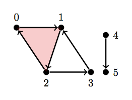
As you can tell this is the same simplicial complex we've been working with except now it has a disconnected edge on the right. Thus we should get Betti=2 for dimension 0 since there are 2 connect components.

H = [{0}, {1}, {2}, {3}, {4}, {5}, {4, 5}, {0, 1}, {1, 2}, {2, 0}, {2, 3}, {3, 1}, {0, 1, 2}]
betti(H)

array([ 2.,  1.,  0.])

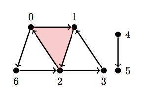
Let's try another one, now with 2 cycles and 2 connect components.
Let \(Y_1 = \text{ { {0}, {1}, {2}, {3}, {4}, {5}, {6}, {0, 6}, {2, 6}, {4, 5}, {0, 1}, {1, 2}, {2, 0}, {2, 3}, {3, 1}, {0, 1, 2} } }\)

Y1 = [{0}, {1}, {2}, {3}, {4}, {5}, {6}, {0, 6}, {2, 6}, {4, 5}, {0, 1}, {1, 2}, {2, 0}, {2, 3}, {3, 1}, {0, 1, 2}]
betti(Y1)

array([ 2.,  2.,  0.])

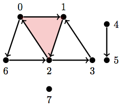
Here's another. I just added a stranded vertex:
Let \(Y_2 = \text{ { {0}, {1}, {2}, {3}, {4}, {5}, {6}, {7}, {0, 6}, {2, 6}, {4, 5}, {0, 1}, {1, 2}, {2, 0}, {2, 3}, {3, 1}, {0, 1, 2} } }\)

Y2 = [{0}, {1}, {2}, {3}, {4}, {5}, {6}, {7}, {0, 6}, {2, 6}, {4, 5}, {0, 1}, {1, 2}, {2, 0}, {2, 3}, {3, 1}, {0, 1, 2}]
betti(Y2)

array([ 3.,  2.,  0.])

One last one. This is a hollow tetrahedron:

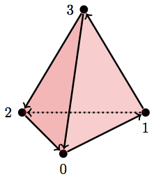
D = [{0}, {1}, {2}, {3}, {0,1}, {1,3}, {3,2}, {2,0}, {2,1}, {0,3}, {0,1,3}, {0,1,2}, {2,0,3}, {1,2,3}]
betti(D)

array([ 1.,  0.,  1.])

Exactly what we expect! Okay, it looks like we can reliably calculate Betti numbers for any arbitrary simplicial complex.

What's next?

These first 4 posts were all just exposition on the math and concepts behind persistent homology, but so far all we've done is (non-persistent) homology. Remember back in part 2 where we wrote an algorithm to build a simplicial complex from data? Well recall that we needed to arbitrarily choose a parameter \(\epsilon\) that determined whether or not two vertices were close enough to connect with an edge. If we set a small \(\epsilon\) then we'd have a very dense graph with a lot of edges, if we chose a large \(\epsilon\) then we'd get a more sparse graph.

The problem is we have no way of knowing what the "correct" \(\epsilon\) value should be. We will get dramatically different simplicial complexes (and thus different homology groups and Betti numbers) with varying levels of \(\epsilon\). Persistent homology basically says: let's just continuously scale \(\epsilon\) from 0 to the maximal value (where all vertices are edge-wise connected) and see which topological features persist the longest. We then believe that topological features (e.g. connected components, cycles) that are short-lived across scaling \(\epsilon\) are noise whereas those that are long-lived (i.e. persistent) are real features of the data. So next time we will work on modifying our algorithms to be able to continuously vary \(\epsilon\) while tracking changes in the calculated homology groups.

References (Websites):

1. http://dyinglovegrape.com/math/topology_data_1.php
2. http://www.math.uiuc.edu/~r-ash/Algebra/Chapter4.pdf
3. https://en.wikipedia.org/wiki/Group_(mathematics)
4. https://jeremykun.com/2013/04/03/homology-theory-a-primer/
5. http://suess.sdf-eu.org/website/lang/de/algtop/notes4.pdf
6. http://www.mit.edu/~evanchen/napkin.html
7. https://triangleinequality.wordpress.com/2014/01/23/computing-homology

References (Academic Publications):

1. Basher, M. (2012). On the Folding of Finite Topological Space. International Mathematical Forum, 7(15), 745–752. Retrieved from http://www.m-hikari.com/imf/imf-2012/13-16-2012/basherIMF13-16-2012.pdf

2. Day, M. (2012). Notes on Cayley Graphs for Math 5123 Cayley graphs, 1–6.

3. Doktorova, M. (2012). CONSTRUCTING SIMPLICIAL COMPLEXES OVER by, (June).

4. Edelsbrunner, H. (2006). IV.1 Homology. Computational Topology, 81–87. Retrieved from http://www.cs.duke.edu/courses/fall06/cps296.1/

5. Erickson, J. (1908). Homology. Computational Topology, 1–11.

6. Evan Chen. (2016). An Infinitely Large Napkin.

7. Grigor’yan, A., Muranov, Y. V., & Yau, S. T. (2014). Graphs associated with simplicial complexes. Homology, Homotopy and Applications, 16(1), 295–311. http://doi.org/10.4310/HHA.2014.v16.n1.a16

8. Kaczynski, T., Mischaikow, K., & Mrozek, M. (2003). Computing homology. Homology, Homotopy and Applications, 5(2), 233–256. http://doi.org/10.4310/HHA.2003.v5.n2.a8

9. Kerber, M. (2016). Persistent Homology – State of the art and challenges 1 Motivation for multi-scale topology. Internat. Math. Nachrichten Nr, 231(231), 15–33.

10. Khoury, M. (n.d.). Lecture 6 : Introduction to Simplicial Homology Topics in Computational Topology : An Algorithmic View, 1–6.

11. Kraft, R. (2016). Illustrations of Data Analysis Using the Mapper Algorithm and Persistent Homology.

12. Lakshmivarahan, S., & Sivakumar, L. (2016). Cayley Graphs, (1), 1–9.

13. Liu, X., Xie, Z., & Yi, D. (2012). A fast algorithm for constructing topological structure in large data. Homology, Homotopy and Applications, 14(1), 221–238. http://doi.org/10.4310/HHA.2012.v14.n1.a11

14. Naik, V. (2006). Group theory : a first journey, 1–21.

15. Otter, N., Porter, M. A., Tillmann, U., Grindrod, P., & Harrington, H. A. (2015). A roadmap for the computation of persistent homology. Preprint ArXiv, (June), 17. Retrieved from http://arxiv.org/abs/1506.08903

16. Semester, A. (2017). § 4 . Simplicial Complexes and Simplicial Homology, 1–13.

17. Singh, G. (2007). Algorithms for Topological Analysis of Data, (November).

18. Zomorodian, A. (2009). Computational Topology Notes. Advances in Discrete and Computational Geometry, 2, 109–143. Retrieved from http://citeseerx.ist.psu.edu/viewdoc/summary?doi=10.1.1.50.7483

19. Zomorodian, A. (2010). Fast construction of the Vietoris-Rips complex. Computers and Graphics (Pergamon), 34(3), 263–271. http://doi.org/10.1016/j.cag.2010.03.007

20. Symmetry and Group Theory 1. (2016), 1–18. http://doi.org/10.1016/B978-0-444-53786-7.00026-5